LiDAR Point Cloud Segmentation: A Novel Approach Using Alpha-Shapes and Voronoi Density Diagrams

Introduction

The high fidelity of LiDAR datasets derived from Terrestrial Laser Scanning (TLS) makes the information type extremely attractive to those that are seeking to model real-world environments in very detailed ways. Sampling densities of ground-based laser scanners can be adjusted to provide for nearly continuous coverage of survey areas, including sub-canopy zone.

In recent years, TLS technologies have become more affordable and the laser scanning systems more user friendly. As a result of these changes, the availability of LiDAR datasets has greatly increased. The challenge for the user of LiDAR data no longer lies in finding ways to get the data, but rather in what to do with all the data that can be obtained.

TLS data is big data. A typical scan captures tens of millions of range measurements and describing the entire shape of an object requires multiple scans. TLS offers up an incredible amount of spatial information, but the data can be difficult to work with because of the size of the files that are generated. Processing tasks can be computationally intensive when carried out on these voluminous datasets and workflows must be methodically designed if projects are to produce results in a timely manner.

In many instances, point clouds contain too much information and objects of interest must be segmented from the larger datasets before they can be worked with. Automating the process of isolating (segmenting) objects of interest from pointclouds is a common LiDAR data management objective and many approaches have been developed.

This research project adds to the existing body of pointcloud segmentation research by proposing a methodology that relies upon alpha-shapes, Voronoi density diagrams, and interpolation methods to extract specific target features, tree stems, from a multi-scan TLS point cloud. The workflow is broken up into two distinct parts. In part one, Alpha-disks are used to identify candidate tree stem bases from a ground point cloud. The results of this stage are then analyzed before moving on to stage two, where point densities and Global Polynomial interpolation methods are used to isolate main stems within the individual tree point clouds.

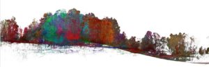
Objects targeted in this segmentation study included main stems of individual blue-gum eucalyptus (Eucalyptus globulus) trees located in the Grinnell Natural Area on the UC Berkeley campus in Berkeley, California. The TLS data used to complete this project was collected over a three-day period in May of 2015. A Faro X130 TLS system was used to collect fifty moderate resolution scans and point cloud registration was carried out using a target-based approach. Project level accuracy for this survey was determined to be at a sub-centimeter level. However, this reported accuracy level can be misleading because it describes the agreement between target points and not points of other objects in the multi-scan pointclouds. The dataset is expected to be far less accurate at the highest elevations because of wind action in the upper portions of tree canopies.

Multi-Scan TLS LiDAR Dataset Processing, Segmentation, Modeling, and Analysis

Processing

Ground points were identified using a binning method that filtered out all points except for those with local minimum elevation values. All points classified as non-ground points were considered to be surface points and stored separately from the ground points. These ground and surface pointclouds were then clipped using a bounding polygon which excluded features present in the study area at the time of data collection that would have complicated the construction of a representative ground surface. Examples of features that were excluded from the dataset used in this study include non-permanent piles of topsoil and stored construction equipment.

In a final preprocessing step a minimum-distance-between-points rule was applied to the surface and the ground pointclouds in an effort to reduce file sizes and make these datasets easier to work with. The minimum distance constraint was set at 25cm for the ground points and 10cm for surface points.

Figure 1. Surface (Top) and ground (Bottom) pointclouds used in this study were created from multiple TLS scans and had minimum-distance-between-points rules applied to them.

Part I

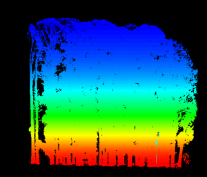
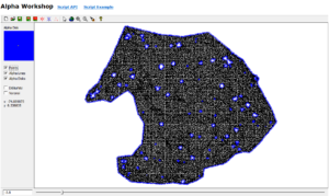
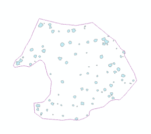
Data holes were present in the processed ground pointcloud (Figure 1 -Bottom). These data holes were exploited in this study for the purpose of isolating individual trees from surface pointclouds. Tree stems created data holes where no ground point measurements existed and candidate tree base outlines were defined by data-no-data interfaces situated within a matrix of ground points. Internal data-no-data boundaries were delineated using nearest neighbor graphs (NNG) created with Alpha-disks. The radii of the Nearest Neighbor graphing Alpha-disks were much smaller than the radii of Minimum Hull Alpha-disks and thus they were able to capture internal structure of pointclouds as well as external extents. Nearest Neighbor Alpha-shapes were constructed using the AEGIS tool.

Figure 2. Minimum Hull (Top) and Nearest Neighbor Graphs (Bottom) were generated from the input ground point cloud using the AEGIS tool.

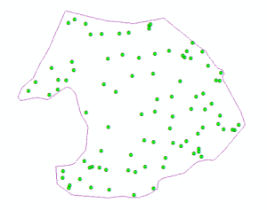
Alpha-lines were exported from the AEGIS software as shapefiles. In ArcGIS, Alpha-line features were converted to polygons using the "Feature to Polygon" tool. A dissolve field was added to the polygons generated from the Alpha-lines and used to merge features that overlapped or shared a common boundary. Centroid-X and Centroid-Y fields were added to the dissolved polygons and the "Calculate Geometry" tool was used to populate these fields. Next, the attribute table of the dissolved polygon feature was exported to a table. The "Display X-Y Data" tool was used to create a point feature from the Centroid-X and Centroid-Y values stored in the exported table. A two-meter buffer was constructed around each of the dissolved candidate tree base polygons. All fields were deleted from the created buffer feature before exporting it as a .dwg CAD file. The CAD file containing candidate tree base buffers was then imported into MapTek's I-Site Studio. The "Filter by Polygon" tool was used to extract out tree points that fell within the XY extents of each buffer feature. This process described in this paragraph can be visualized in Figure 3.

Figure 3. Nearest Neighbor Graphs representing candidate tree bases were converted to polygons (top). The centroids of these polygons were located (second down from top) and then 2-meter buffers were created around them (third down from top). These buffer features were then used to clip out LiDAR points from the input surface point cloud (bottom).

Separate point clouds were created for each buffer extracted feature from the surface pointcloud and examined to confirm the presence of a tree base at the site of each buffered feature's centroid. If a pointcloud contained a single stem at ground level, it was given a rating of good. If a pointcloud contained more than one stem with one surrounding the centroid at ground level, it was given a rating of satisfactory. And if the pointcloud contained no stems at ground level then it was given a rating of poor. For this study, trees with the rating of good were then focused on in Part II.

Part II

Once a point cloud containing a single, nearly complete tree was segmented out of the surface pointcloud an effort was made to remove branches that were close to the main stem of the tree. This was done by projecting the entire pointcloud onto an XY plane and then searching for areas of high density. This approach rested upon an assumption that main stems would be located in areas of highest point density when only X and Y coordinates were taken into account. This density based approach to pointcloud segmentation also relied on dataset dimension reduction. 3D pointclouds were projected onto 2D planes and that plane was then segmented into polygonal regions using Voronoi diagrams. The weighted density of each Voronoi diagram delimited cell was then attributed to the planar-projected LiDAR points that fell within that cell using a spatial join function in ArcGIS. Voroni Density Diagrams were constructed using scripts in the UC Berkeley LAEP C177 course toolbox written by Daniel Radke.

Figure 4. An individual tree pointcloud is projected onto a XY plane (left). Note the large number of data points that are located in the main stem region of the pointcloud (right).

In order to isolate all individual-tree points within regions of high point density, clipping polygons were created to filter out all points that did not meet a minimum density criteria. This was accomplished by building continuous Global 5th-order polynomial interpolated raster surfaces in ArcGIS that estimated Voronoi point densities across entire dimensionally reduced individual-tree point clouds. The classification break values were then adjusted to bound regions of target point densities. High point density regions were then reclassified and converted to polygons. An additional processing step was added before the raster was converted to polygons which removed edge effects by clipping the interpolated surface with a Minimum Hull Alpha-shape constructed in the AEGIS software. High point density delimiting polygons were exported as CAD files before being used as filtering objects in MapTek's I-site Studio.

Figure 5. A Global 5th-order polynomial interpolated raster surface generated in ArcGIS which estimated Voronoi point densities across the entire dimensionally reduced individual-tree point cloud. The purple line is the Minimum Hull Alpha-shape constructed in the AEGIS software from the individual-tree point cloud and used to eliminate edge effects on the final interpolated surface.

Results

Part I yielded many interesting results. The NNG alpha value of -3.8 was very low compared to the Minimum Hull alpha value of -1.1. The NNG did a good job of capturing candidate tree stem bases while excluding non-candidate gaps in the ground pointcloud. 120 polygons were created from the conversion of the NNG Alpha-lines to polygons. After dissolving overlapping and connected polygons, the total number of candidate tree stem bases dropped to 90. When the buffered dissolved polygons were used to filter individual trees from surface point clouds, the results were mixed. 23 buffered candidate tree stem bases did a poor job of capturing any tree stem material. 17 buffered candidate tree stem bases did a good job of capturing any tree stem material. The remaining 50 buffered candidate tree stem bases did a satisfactory job of capturing tree stem material. Examples of outputs from part one can be examined in Figure 6.

Figure 6. Examples: Good job of capturing tree stem material (Top); Satisfactory job of capturing tree stem material (Middle); Poor job of capturing tree stem material (Bottom).

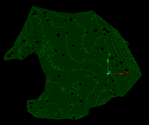
Part II seemed to produce promising outcomes. However, time limitations allowed for only a small number of individual-tree point clouds to be put through this stage of testing. One exciting result has been visualized in Figure 7, which shows the Voronoi density values attributed to the individual LiDAR points. There are marked increases in densities in areas where tree stems are present in the point cloud. This provides evidence to support one of the key assumptions of this approach to individual tree stem segmentation.

Figure 7. 3D individual-tree point cloud projected onto an XY-plane. YZ and XZ planes (Left) display the Voronoi density values that have been attributed to individual LiDAR points. YZ and ZY planes (Right) display the height values of these points.

Generating the Global 5th-order polynomial interpolated raster surface to estimate Voronoi point densities across the entire dimensionally reduced individual-tree point cloud also seemed to be an effective component of the proposed approach to main stem segmentation from an individual-tree point cloud. The high density region captured nearly all of the stem points and lopped off many of the branches. Figure 8 shows point cloud that was extracted using the polygon filter created from the interpolated surface.

Figure 8. The yellow 2D object was a classification boundary generated by the Global Polynomial Interpolation and used to extract points from high density regions of the individual tree point cloud. These points have been heat mapped according to their elevation values and are shown on the right side of the figure against a black backdrop.

Discussion and Concluding Remarks

There are many reasons to be excited about the potential of this point cloud segmentation method. It is all based on point densities and XYZ-coordinates, which means all the information that is needed to carry it out is already contained in the most basic of TLS datasets. The segmentation method does not require any additional data inputs and this may prove to be its most redeeming quality. The method also could be scripted and the process could be partially automated. Even satisfactory results could represent huge time savings when it comes time to classify and segment large point clouds.

There is also reason to believe that the process can be improved by fine tuning the buffer sizes so that they do a better job of capturing only main stem points that belong to their respective candidate bases. In areas where tree stems are more clustered or grow more straight in the vertical direction, it would make sense to use a smaller buffer size. In places where trees have exaggerated sweeps it would make sense to use larger or more elliptical buffers.

In cases where this method did a poor job of capturing tree stem material, it appears that there may be some systemic error at work. All of the poor outcomes are positioned at the very exterior of the study area. This could mean that non-target trees were removed from the surface pointcloud but their presence was still detected by a gap in the ground point cloud. This explanation could be easily confirmed or rejected by looking back at the original scans and seeing if there are any trees that have been removed within the extent of the surface point cloud.

Figure 9. The centroids of all candidate tree bases. Black dots did a poor job of capturing tree stem material, grey dots did a satisfactory job, and gold dots did a good job.

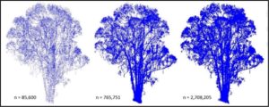
Data subsetting is of paramount importance when working with dense TLS data. It is wise to use as few points as is needed to observe a variance in density that could be associated with large features in the tree pointcloud if computational resources are limited. It is also good to keep in mind that points falling close to these defining nodes can be called back in to the pointcloud when a need arises to make use of LiDAR's phenomenal spatial coverage and positional accuracy.

A successful LiDAR data workflow is likely to fall into the pattern: subset points out of point cloud, explore less data heavy pointcloud, isolate or measure objects, and repopulate some points to these isolated point cloud segments to increase the resolution of the dataset segment. Real gains in time and stress relief are made by having fewer points to project on the fly as you visualize TLS datasets and try to extract meaning from them. Segmentation is key to the usefulness of LiDAR and methods that meet this data management objective can be invaluable when projects are scaled up to larger regions of interest.

— Liam Maier
Digital Reality Architect